Spatial Transcriptomics FAQs

Introduction

Spatially resolved transcriptomics (SRT) is a cutting-edge scientific method that merges the study of gene expression with precise spatial location within a tissue. This revolutionary approach allows researchers to visualize the spatial distribution of RNA transcripts within a tissue sample, essentially mapping out where each gene is being expressed. Traditional transcriptomics analyses gene expression in bulk tissue samples or single cells but lacks spatial information.

Polly can bring in SRT data from a variety of public sources as per the needs as long as the raw counts matrix, spatial coordinates, imaging data, and metadata are available. Some of the common public sources for Spatial Transcriptomics data are:

1. Gene Expression Omnibus
2. Single Cell Portal
3. Zenodo
4. CZI-CellxGene
5. Publications

How is a spatial transcriptomics dataset on polly defined?

Spatial Transcriptomics Datasets on Polly represent a curated collection of biologically and statistically comparable samples. Each dataset is denoted using a unique ID, whose nomenclature depends on the public database it was ingested from.

Spatial datasets are stored in a sample-wise fashion, i.e. multiple samples from a series are hosted as individual datasets. This is done as often publications have been observed to analyze individual samples independently due to lack of a straightforward way to combine spatial coordinates and imaging data from distinct tissue sections.

Source	Source Format	Polly Format
GEO	For every study, there is a series ID and a sample ID given on GEO. Series - A Series record links together a group of related samples and provides a focal point and description of the whole study. Each Series record is assigned a unique GEO Identifier (GSExxx). A Series record can be a SubSeries or SuperSeries. SuperSeries is all the experiments for a single paper/study and is divided into SubSeries which are different technologies. Sample - A Sample record describes the conditions under which an individual Sample was handled, the manipulations it underwent, and the abundance measurement of each element derived from it. Each Sample record is assigned a unique and stable GEO accession number (GSMxxx)	Format: GSExxxxx_GSMXXXXX
Single Cell Portal(SCP)	Studies on SCP have a unique ID associated with them. Eg. SCP2331	Studies fetched from the Single Cell Portal follow the same nomenclature as that of the source. The unique dataset ID format is SCPxxxxx Eg.SCP2331
Zenodo	Zenodo hosts “records”, which are the basic entities used to share and preserve a digital research object (datasets, publications, software, poster, presentations etc). Each record on Zenodo has a unique Digital Object Identifier (DOI) associated with them Eg. 4739738	Studies fetched from Zenodo follow the same nomenclature as that of the source. The unique dataset ID format is for ex. 4739738
CZI-CellxGene	Datasets on CZI have a unique alphanumeric ID associated with them. Eg. 60358420-6055-411d-ba4f-e8ac80682a2e	Studies fetched from CZI follow the same nomenclature as that of the source. The unique dataset ID format is for Eg. 60358420-6055-411d-ba4f-e8ac80682a2e
Publication	-	Studies for which data is taken from publication directly (not from the above sources) are available with a unique dataset ID as the PMID of the paper. Eg. PMID35664061

What are the different options within the Spatial datasets on Polly?

Currently, Polly provides Spatial datasets generated using 10X Genomics’ Visium technology. To be noted, the sampled entities for Visium datasets are “spots” (which may contain 10-30 single cells) rather than individual cells. We offer spatial datasets in two formats - Curated raw unprocessed datasets and Curated custom processed datasets

Raw unfiltered counts

This format contains one H5AD file containing raw counts for unfiltered spots and genes as the data matrix, spatial coordinates of the spots, H&E image of the tissue section used for generating the data, curated sample level metadata, and normalized feature names. More details are in the subsequent sections. This format is useful if the research needs raw counts to be processed in a custom manner.

Custom processed counts

This format contains 2 H5AD files.

a. One H5AD file is the same as mentioned in the Raw unfiltered counts section

b. The second one stores the following in addition to fields in the raw data

• Processed counts using a pipeline for filtering spots/genes, normalizing the counts must be as per requirement
• Raw counts after filtering out the spots and genes as per requirements.
• Normalized and log1p transformed counts.
• Results from dimensionality reduction and clustering of spots
• Results from spatially variable genes (SVG) analysis
• Results from cell type deconvolution using associated reference single cell data.
• Curated sample-level metadata and normalized feature names.

The pipeline uses default standard parameters at every processing step which can be customized as per requirement. However, methods used for SVG and cell-type deconvolution are currently fixed.

Details

1. Raws unfiltered counts

1.1. Starting Point

To process spatial transcriptomics datasets using Polly's pipeline, the starting point is a counts matrix in h5 format, spatial coordinates (of the spots) provided in csv format, both low-resolution and high-resolution H&E images of the tissue section used for data generation, a scalefactors JSON file for the mapping of spot coordinates to image pixels, curated sample-level metadata, and normalized feature names.

1.2 Processing details

The pipeline for raw counts includes the following steps:

1. Fetching Raw Counts: The starting point for the pipeline is getting the raw counts and spatial data from the source by

   • Either downloading data directly from the source
   • A text file is created with links for downloading
   • Downloading manually

2. Preparing Data files: A JSON file is created for the pipeline to run.

   • A JSON file containing all necessary input parameters is generated. Subsequent steps in the pipeline are executed based on the parameters specified in this JSON file.

3. Creating h5ad: With the input as the above JSON file, the pipeline starts to create the initial h5ad.

   • Programmatic checks are performed to ensure that counts data, spatial coordinates and required image files (tissue_hires and lowres images, scalefactors.json) are available.
   • Check that the data matrix contains raw counts only
   • If the matrix is not found to be in the correct format (as per the raw count acceptable values), the pipeline stops
   • Pipeline accepts the raw counts as per defined the acceptable values, i.e. integer values
   • The index for spot data is “cell id” which is in the form of “sample id : spot barcode” and information with respect to each “cell id” is added
   • Feature IDs are converted to Hugo Symbols (or Ensembl IDs where conversion to Hugo symbols is not available or ambiguous)
   • Initial h5ad is created

4. Metadata Curation:

   • The curation pipeline adds curated metadata to the file - sample/cell level metadata is added to the h5ad file
   • The curation pipeline generates dataset metadata

5. QC metrics: Scanpy QC metrics are calculated and added to the h5ad file

6. Spatial Embedding for visualization with cellXgene: A X_spatial embedding is added to the h5ad obsm slot. This is a copy of the spatial embedding which is added automatically when creating the initial h5ad.

7. Final h5ad: The final h5ad file is saved, consisting of QC metrics, curated metadata, raw counts matrix, spatial coordinates and H&E images.

1.3 Curation and Metadata details

On Polly, every dataset and its corresponding samples are tagged with some metadata labels that provide information on the experimental conditions, associated publication, study description and summary, and other basic metadata fields used for the identification of dataset/samples.

There are three broad categories of metadata available on Polly such as:

a) Source Metadata: Metadata fields that are directly available from the Source and provided in a Polly-compatible format.

b) Polly - Curated: These are curated using Polly’s proprietary NLP-based Polly-BERT models and reviewed by expert bio-curators to ensure high-quality metadata. Some of the Polly curated metadata fields are harmonized using specific biomedical ontologies and the remaining follow a controlled vocabulary.

c) Standard identifiers - Identifier metadata tag for datasets, giving information on the basic attributes of that dataset/study.

Metadata for every dataset is available at 3 levels:

I) Dataset-level metadata - General information about the overall experiment/study, for eg, organism, experiment type, and disease under study.

II) Sample-level metadata - Information about each sample related to Eg. Drug, tissue.

III) Feature-level metadata: Information on the genes/features that are consistent across samples.

1.4 Output H5AD format and details

H5AD file for raw counts data offering will be available to the user with the following information:

1. Raw counts <adata.X> slot: The raw expression matrix is available in this slot, providing information on the genes and cells as provided by the author. The raw counts will available be as:

   • Integer counts (with an exception of some datasets from Expression Atlas which may contain fractional values)
   • Values not less than 0
   • Sparse matrix

2. Spatial Coordinates data: Columns in_tissue, array_row, array_col are available in the <adata.obs> slot.

   • in_tissue column: indicates whether the spot falls under the tissue section
   • array_row and array_col: provide location of each spot on the Visium array
   • Pixel coordinates for the spots (for plotting spots on the image) are added as a 2D array to the slot (key: spatial)

3. A “X_spatial” key is added to <adata.obsm> slot. This contains exactly same info as adata.obsm[“spatial”] which is automatically added upon creating the h5ad. It is required for compatibility with downstream visualization packages.

4. Imaging Data: Image data is added to the <adata.uns>. The “spatial” key in the uns slot holds a dictionary containing lowres, hires image arrays and scalefactors used for mapping spot coordinates onto the lowres/ hires images.

5. Complete Sample Metadata in <adata.obs> slot: All the spot/sample level metadata information is available in this slot as per the metadata table given above

   • Polly-Curated Metadata
   • Scanpy QC metrics - QC metrics include n_genes_by_counts, total_counts, total_counts_mt, and pct_counts_mt.
   • Source Metadata
   • Standard Identifier Metadata

6. Processing Details <adata.uns> slot: Unstructured metadata on the processing-related details is available in this slot such as:

   • Tools/packages along with their versions used to convert the matrix from source to H5AD file
   • ontology version
   • raw file formats
   • scanpy, anndata version

7. <adata.uns> slot: QC Metrics such as mt, n_cells_by_counts, mean_counts, pct_dropout_by_counts & total_counts

2. Custom Processed Data

2.1. Starting point

For processing SC datasets using the customizable pipeline, the starting point is a h5ad file containing either raw unfiltered counts, QC filtered counts or normalized counts. The inputs for the processing pipeline are:

• The H5ad file should contain required spatial coordinates, images, and sample/spot and feature level metadata. Features should be HUGO gene symbols as feature IDs.

• Reference single cell RNA-seq dataset for performing cell type deconvolution. Can be provided as a text file containing links to the raw data and cell label metadata.

2.2. Processing details

1. Preparing files

• A JSON file is created with all the required input parameters for the processing workflow.
• This should include a dataset id for the reference single cell dataset to be sourced from sc raw omixatlas and used for deconvolution.

2.Processing Workflow:

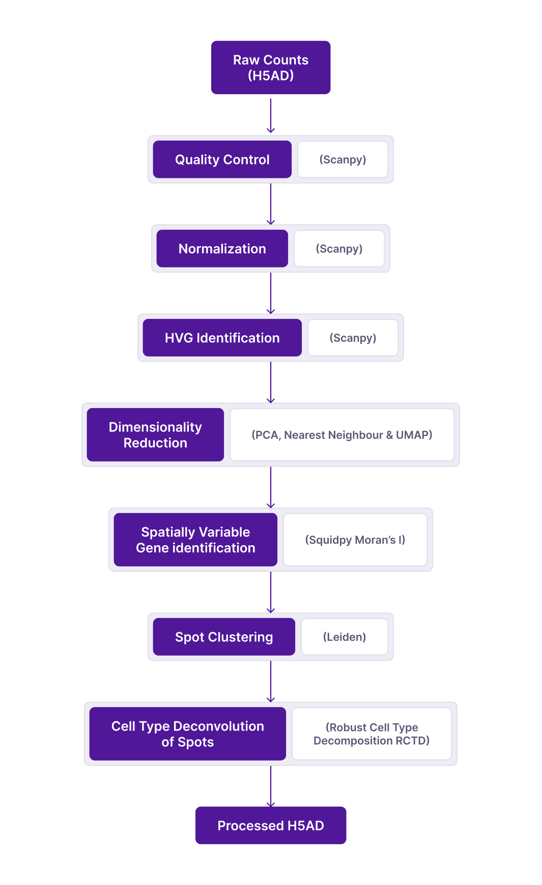
Spatial data is treated as single cell data for QC and some downstream analyses. Standard pipeline workflow consists of the following steps guided by following the single cell best practices guide by default with additional customization as options.

a. Data Checks

Data checks are done such as

• X contains raw counts
• X is a sparse matrix in csr_format
• mt, ribo, and hemo tags are added to genes
• Copy of unfiltered counts matrix from X to raw slot
• obsm contains spatial & X_spatial embeddings
• uns contains spatial dictionary with image arrays and scalefactors

b. Quality Control

With the gene expression matrix ready (raw counts matrix), the next step is to filter out low-quality cells and genes before further processing. Following the best practices guide, filtering of cells is done using adaptive cutoffs per dataset

• Spot filtering

Following the best practices guide, we use ratios instead of hard thresholds. This adapts cutoffs according to the distribution in each dataset. Outlier spots crossing at least one of the following thresholds are removed (MAD is median absolute deviation)

• log1p_total_counts > or < 5 MAD,
• log1p_n_genes_by_counts > or < 5 MAD,
• pct_counts_in_top_20_genes > or < 5 MAD,
• pct_counts_Mt > 3 MAD and > 8%
• Gene filtering: genes expressed (counts > 0) in less than 3 cells are removed

c. QC metrics calculation

QC metrics are calculated for ribo & hemo genes as well, but genes are not removed based on these metrics.

d. Normalization

Normalization is performed to reduce the technical component of variance in the data, arising from differences in sequencing depth across spots. It is performed based on the following best practices :

• Method: library size/total counts normalization (implemented by scanpy.pp.normalize function)
• target_sum: None (this is the default option in scanpy and amounts to setting the library size to the median across all cells; best practices guide discusses the use of alternate fixed thresholds like 10^4 or 10^6 can introduce over-dispersion)
• log1p: True
• Scaling: True, with zero_center=False (this will be performed after the HVG step)

Note: Before normalization, the filtered counts matrix is saved to a separate “counts” layer (adata.layers["counts"]), and X is updated with the normalized counts matrix. A copy of the normalized (and optionally log1p) counts matrix will also be saved in a separate “normalized_counts” layer, this will preserve the normalized data prior to scaling.

e. HVG identification

Feature selection is needed to reduce the effective dimensionality of the dataset, and retain the most informative genes for downstream steps like PCA and neighbor graph

• Highly Variable Genes (HVG) are identified using the scanpy.pp.highly_variable_genes function with the following settings:

• HVG method: "Seurat" (default, uses the log-normalized counts matrix in X)

• n_top_genes (# HVGs identified): 2000
• subset: False - the expression matrix is not subsetted to the HVGs. All genes are retained and a highly_variable column gets added to the .var slot

f. Dimensionality reduction

This step is necessary to reduce the dimensionality of the data prior to clustering, and to enable visualization for exploratory analysis. Following data embeddings are provided by running the relevant scanpy functions:

• PCA (n_pcs = 50 top PCs ranked by explained variance): 'X_pca' in obsm, 'PCs' in varm slot
• Nearest-neighbor graph in PC space: n_neighbors=50, dimensionality of PC space = 40 or number of top PCs explaining 90% variance, whichever is smaller; 'distances' and 'connectivities' in obsp slot
• Uniform Manifold Approximation and Projection (UMAP): 'X_umap' in obsm slot

g. Spot clustering

Unsupervised clustering is performed on the processed and dimensionally reduced data matrix to identify similar groups of spots, possibly representing distinct cell compositions/states.

• Leiden graph-based clustering is performed with a fixed resolution (resolution = 0.8)
• The nearest-neighbor graph is constructed in the previous dimensionality reduction step.
• Cluster labels are added to the obs slot in a ”clusters” column

h. Spatially Variable Genes Identification:

Spatially variable (SV) genes are genes whose expression distributions display significant dependence on their spatial locations. SV genes are often markers or essential regulators for tissue pattern formation and homeostasis.

• Spatially Variable Genes are identified using the squidpy.gr.spatial_neighbors and squidpy.gr.spatial_autocorr functions run in that order.
• The mode parameter in squidpy.gr.spatial_autocorr function is set to “moran”.
• A matrix Spatial_neighbors is added to Uns slot
• moranI dataframe containing I statistic, p-val, p-val-corrected is added to Uns slot
• spatial_distances and spatial_connectivites matrices are added to Obsp slot

i. Cell type Deconvolution of Spots:

Cell type deconvolution is performed on spatial transcriptomics data in order to dissect the cell type compositions within each spot.

This is done using a reference single cell dataset already annotated with cell type labels using the deconvolution metho - RCTD. The tool we are using for deconvolution is RCTD. This is a reference based deconvolution tool, i.e. it requires a reference single cell rna seq dataset, which has celltype annotation. The tool was selected as it operates fast, is not computationally intensive, works with raw counts for reference and query (spatial) data, and has been found to be fairly accurate with real data compared to other tools in the same category.

• RCTD - Input

  • A reference object is created using RCTD’s Reference function, which requires a cell x gene matrix of raw counts, a named vector of cell type labels, and a named vector of total counts in each cell.
  • A query object is created using RCTD’s SpatialRNA function, which requires a spot x gene raw counts matrix, a dataframe of spatial coordinates and a named vector of total counts in each spot.
  • The create.RCTD function is used to create an RCTD object using the reference and query objects
  • The RCTD object is supplied to the run.RCTD function to perform cell type deconvolution specifying mode = “full”

• RCTD - Output

  • run.RCTD returns the RCTD object containing deconvolution results in the @results field. Of particular interest is @results$weights, a data frame of cell type weights for each spot (for full mode).
  • The @results$weights dataframe is normalized (such that each row sums to one) using the normalize_weights function
  • The main cell type assigned to each spot is computed as the cell type with the highest proportion in the spot.

• Annotated Tags:

• Following sample-level metadata columns get added to obs (these would be uniform across all cells in each cluster):

  • polly_curated_cell_type: Raw cell type associated with the cell
  • polly_curated_cell_ontology: Cell type associated with the cell, curated with standard ontology
  • Following outputs of the cell annotation step are saved to the uns slot of the anndata object:
    • The full dataframe of normalized cell type weights for each spot.

j. Saving the data

The parameter dictionary will be saved to the uns slot, after adding a time stamp as the “time_stamp” key to the params dict. The X matrix will be converted to csc_matrix format and the processed anndata object will be saved in H5AD format and pushed to Polly’s omixatlas. Further, details of the processing performed (parameters/method choices, QC metrics, and associated plots) are bundled as a separate comprehensive HTML report and provided along with the data file.

2.3. Curation and Metadata details

Metadata curation for Polly annotated data is the same as raw counts data (given above). However, there are some additional fields that are present for custom-processed dataset in addition to the existing fields available for raw unfiltered data.

Details on each metadata field present at the dataset, sample, and feature level are given here.

2.4 Customization

The tools and parameters for processing datasets as per Polly’s processing pipeline are standard. Any changes will be considered a custom request. There are some guardrails such as:

• QC filter (choice between fixed cutoffs vs best-practices adaptive cutoffs per sample or across all datasets)
• Gene filter cutoff (# of cells expressed)
• Filtering of gene groups (mitochondrial (mito)/ribosomal (ribo)/hemoglobin (hb))
• Normalization: Size factor (value), log1p (true/false), scaling (true/false)
• HVG selection: No. of highly variable genes (value), dispersion method
• Scaling (true/false) and zero centering (true/false)
• Regressing cell covariates ( none, covariates )
• Embeddings: # of PCs, # of neighbors for neighborhood graph and clustering
• Clustering: Resolution parameter, Method (Louvian/Leiden)
• Spatially Variable genes - autocorrelation method (moran/ geary C)

No customization is currently offered for cell type deconvolution

2.5. Output format and details

Two H5AD files will be made available to the user.

1. Raw unfiltered counts data (Details given above)
2. Custom Processed data: _custom_processed.h5ad

The following information will be available in the H5AD file (Dataset_id>_polly_annotated.h5ad)

1. Raw filtered counts in <adata.raw> slot: The expression matrix after filtering out the genes and cells as per Polly's standard processing pipeline is available in this slot

   • Integer counts
   • Sparse matrix

2. Processed filtered counts in <adata.x> slot: The expression matrix after filtering out the genes and cells and normalising the counts as per Polly's standard processing is available in this slot as:

   • Float values
   • Values < 100
   • Sparse matrices

3. Complete Sample Metadata <adata.obs> slot: All the sample/cell level metadata as per the metadata table given above is available in this slot. This includes

   • Polly-Curated Metadata
   • QC metrics
   • Source Metadata
   • Standard Identifier metadata
   • Spatial Coordinates Metadata

4. Embedding data in <adata.obsm> slot. This includes the following:

   • PCA: Principal components minimum
   • NN: Nearest Neighbour graph
   • UMAP: Coordinates of the UMAP plot
   • Spatial: Pixel Coordinates for each spot
   • X_Spatial: Copy of Spatial for compatibility with cellxgene visualization

5. Unstructured metadata in Uns slot: This includes the following:

   • A dictionary containing lowres, hires image arrays and scale factors
   • A matrix of Spatial_neighbors
   • moranI dataframe containing I statistic, p-val, p-val-corrected from the SV Genes analysis
   • Tools/packages along with their versions used to convert the matrix from source to raw counts H5AD file
   • Tools/packages along with their versions used to convert the raw counts H5AD file to custom processed counts H5AD file
   • processing pipeline version
   • curation model version (for eg. PollyBert_v1)
   • ontology version
   • squidpy, scanpy, anndata version
   • Parameters used for processing the data (as a dictionary)
   • Table of sample-wise QC stats (no. of cells pre/post filtering, along with filtering thresholds applied)
   • A dataframe of cell type proportions from the deconvolution analysis

6. Pairwise annotation of observations in Obsp slot:

   • Spatial_connectivities matrix created during SV genes analysis
   • spatial_distances matrix created during SV genes analysis